K-cores Decomposition of a Real Network

Let’s now consider a real network. The Internet is a very complex system and its rapid growth makes its graph representation very interesting, from a topological point of view. Many projects tried to map the Internet and this implies all kinds of difficulties. DIMES project has the peculiarity of being a collective effort, it is a distributed scientific research project, aimed to study the structure and topology of the Internet, with the help of a volunteer community. What you have to do to participate and become an Active Agent is to download a small program that will run in the background of your computer, consuming very little resources. The network considered for this post is the result of the data gathered from 2004 to 2007, it has 34563 vertices and 62960 edges, with a maximum degree of 2897. In particular this is the Autonomous System (AS) level of the Internet network. Each vertex represents an autonomous system and each edge is a connection between two AS. That is why it may seem small, but every vertex is a collection of routers and networks under the same domain or administrative entity.

Dimes AS Network Degree Distribution

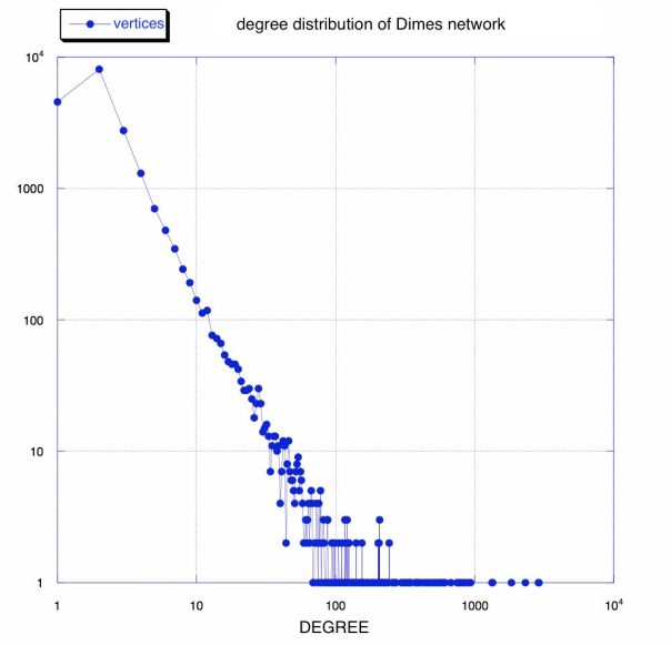
I already mentioned here the first characteristic of complex networks, the scale invariance with the typical power-law distribution of degrees. We can see in the picture above that in this case we have indeed a power-law with an exponent of 2.5 and a long exponential tail.

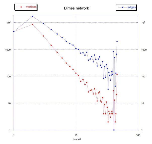
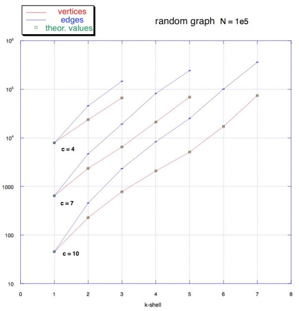
We observed here that for a random graph we have a Poisson distribution of degrees and consequently an homogeneous topology. We may expect now something quite different. How does this k-cores decomposition look like? We can see below in red the distribution of vertices, and in blue the edges, that is the number of vertices and edges in each shell. It seems the opposite of what we saw for random graphs. Most vertices are in the lower shells, and few are very connected. The number of elements in each shell decreases with k. In particular the number of vertices decreases with k following a power-law with an exponent of 2.7.

Dimes Network with 34563 vertices and 62920 edges, k-cores decomposition

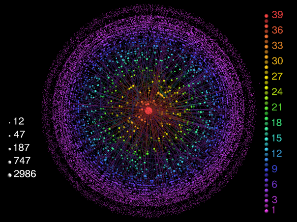
In the figure below these characteristics become even more clear. This very nice image is obtained with the LaNet-vi visualization tool, mentioned in the previous post and described here. The size of a vertex represents its degree and the color represents its coreness value (or the shell where the vertex is). This graph has clearly an heterogeneous topology, there is an evident hierarchy, most vertices are in the lower shells, pink and purple, whereas a limited number of vertices has an important role in the network, in the center of the picture. These red vertices are called hubs and they have a very large number of connections. Emergence of hubs is a consequence of the scale-free property of networks. Hubs can be found in many real networks and have a significant impact on the topology, but they cannot be observed in a random network, as we already saw.

How this network would resist to damages and attacks? We already saw that removing a random vertex in a network with an homogeneous topology like a random graph we probably would not cause much trouble, because those vertices have a similar role in the network, they are interchangeable. Here instead, we have a group of nodes that are essential, without one of them we would probably find our network divided in disconnected components or clusters. Here of course, removing a random element means to touch more likely one of the less important vertices, but we have a part of the network very sensitive and an attack towards one of the red vertices would have serious consequences. This example of an highly hierarchical network shows us why local failures don’t usually lead to catastrophic global failures. Scale-free networks are resilient with respect to random attacks, whereas targeted attacks are very effective.

k-cores decomposition visualization by LaNet-Vi

K-cores Decomposition of a Random Graph

We described what cores are and it is now time to see how a network looks like, once we performed the k-cores decomposition. There is a very interesting visualization tool for graphs called LaNet-vi and it is based on the k-cores decomposition, described in previous posts here and here. This visualization tool provides very nice images of large scale networks on a two-dimensional layout.

Let’s consider first a random graph with N vertices and M edges. A random graph is obtained by a stochastic process that starts with N vertices and no edges, and at each step adds one new edge chosen uniformly with probability p from the set of missing edges. The number of possible edges is N (N – 1), that is the number of edges of a complete graph. A random graph with N vertices and M edges has an average degree c = 2 M / N, and the degree distribution follows a Poisson probability distribution. As we saw before, the k-core decomposition depends strongly on how the edges are distributed among the vertices.

The theory of random graphs says that there is a critical threshold c(k): if c ≥ c(k) then the k-core exists and it is formed by a finite group of vertices. I generated several random graphs for c = 4, 7, 10 and I performed the k-cores decompositions, writing some code in C programming language. In the plot below we can see the number of edges (in blue) and the number of vertices (in red) that belong to a k-shell (the vertices and edges that belongs to the k-core but not to the (k+1)-core ) with a value of coreness k. The green small squares represent the theoretical values for random graphs, given c and N. If you are interested the code is available in my repository here under the KCores folder.

Random Graph with 10^5 vertices

How does this k-cores decomposition look like? And how is this useful? We notice that most of the vertices and edges belong to cores with high value of k. And also that the number of elements in a shell grows with k. And when c grows, new cores with larger k appear, as we expected from random graph theory. In the figure below these characteristics become even more clear. This very nice image is obtained with the LaNet-vi tool, mentioned above. This random graph has 1000 vertices and an average degree c = 10. The size of a vertex represents its degree and the color represents its coreness value (or the shell where the vertex is). This graph has clearly an homogeneous topology, there is no evidence of hierarchy, most of the vertices share the same role in the network (in red in the picture below). Often we read about the strenght of a network, that is how a network resists to damages or attacks. In this case, with an homogeneous structure, if we remove a random vertex or edge, we probably would not cause much trouble to this network, because most vertices are connected to each other and share the same role. This means that a random graph has a strong structure. And, obviously, this is the exact opposite of what we have in real networks.  But we will see what happens in real life in the next post!

k-cores decomposition visualization by LaNet-Vi

K-pruning Algorithm

We want to highlight in a graph some subsets with important connectivity properties, the cores. We described what these cores are in detail in a previous post. But how do we break down a graph in its cores? To partition the graph there is an interesting recursive algorithm, called k-pruning and I will describe here how it works. I also wrote some code in C programming language, to perform this decomposition on a general undirected graph, given its representation as a list of edges in a text file. 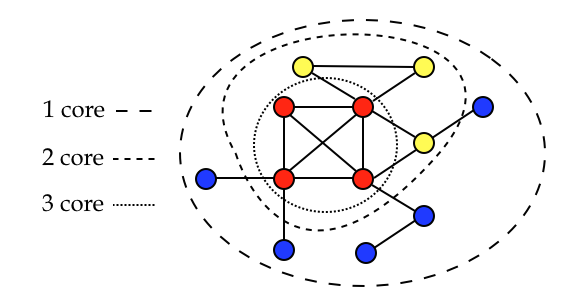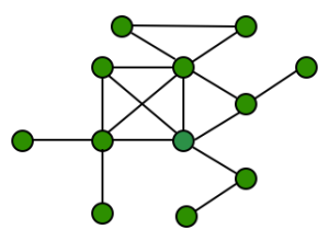If you are interested you can find this C code here in my repository (under kCores folder).Let’s now consider a cyclic undirected graph, green vertices in the figure above. From the definition of k-core we have that every vertex with degree ≥ k belongs to the k-core. We notice that every vertex in this graph has degree ≥ 1, thus the whole graph should be a 1-core.

The algorithm of the k-pruning says: remove recursively all vertices with degree < k, the remaining vertices belong to the k-core.  In order to have all the possible cores of the graph, we have to perform this recursive pruning for k going from the minimum degree of the graph to the maximum degree. In this case we have minimum 1 and maximum 6. According to this procedure, we can see that there are no isolated vertices, with degree < 1, thus the whole graph is a 1-core, as we already noticed.

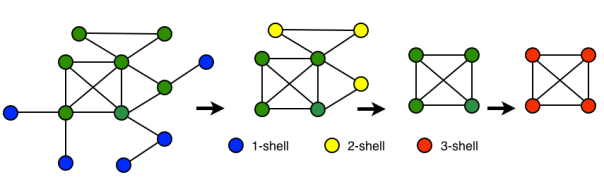We now remove recursively all vertices with degree < 2, the vertices in blue in the figure above. We obtain the 2-core (remaining green vertices). The blue vertices belong to the 1-core but not to the 2-core, thus they are the 1-shell (see here for definitions and more details). Same happens for the vertices with degree < 3, in yellow in the figure above. They are removed recursively and we obtain the 2-shell, and the remaining vertices belong to the 3-core. We notice now that removing all vertices with degree < 4 we have nothing left. That means that the we have no more inner cores to find.

We did not perform the pruning for all values of allowed k, from minimum degree 2 to maximum degree 6. With degree 4 we already found no vertices left. This gives us an idea of how many and strong connections should be in a graph, in order to resist to a pruning with an high value of k. Therefore the core decomposition of a graph gives us very different results depending on the degree distribution.

K-cores Decomposition of a Graph

The Graph is a really beautiful and useful mathematical object, with many properties. Before introducing the k-cores, let’s describe shortly some basic principles. In general a graph is defined by a set of vertices and edges that connect pairs of vertices. Usually N represents the total number of vertices and M the number of edges. The degree is the fundamental characteristic. Every vertex has a degree, that is the number of edges that connect that vertex  with the others. With the same N and M we can build very different graphs, depending on the degree distribution, that represents how the edges are distributed among vertices.

Moreover graphs can be trees, which means without loops, or closed paths. Otherwise they are cyclic graphs, if they have at least one loop. The path from a vertex v to another vertex w is a sequence of connected vertices, where no edges or vertices are repeated. A loop is simply a path that starts and ends with the same vertex.

Example of a tree

A complete graph or fully connected graph, is a graph where every vertex is connected with all the others. If we have N total vertices, we will have all vertex with degree N – 1. Which means that we can go from everywhere to everywhere in just one step. Real networks usually do not have this super property, but they may have some highly connected parts. A clique in a graph is indeed a subset of vertices where every vertex has the maximum possible degree, in other words a complete graph inside another graph. In the example below in the 2-clique all vertices have degree 2, in the 3-clique all vertices have degree 3 and so on.

Example of n-clique

Let’s go further. A graph is k-connected if every pair of vertices is connected through at least k distinct paths, that do not share edges. This property is related to the strength of a network, in fact a k-connected network remains connected whenever fewer than k links are removed or broken.

Now we can finally introduce the k-core, also related to the strength of a network. The k-core is a subset of a graph where every vertex has degree ≥ k. Cores are nested, a graph can have a 2-core that includes a 3-core that includes a 4-core and so on. Every vertex of a graph has its coreness value, that represents the maximum k-core that contains it. In other words a vertex has coreness 3 if it belongs to the 3-core but not to the 4-core.  The k-shell is the subset of vertices with the same value of coreness. We can see now that cliques are always also cores. The opposite is not true, cores are not necessarily cliques.

In the example below we have a graph with its cores decomposition.  The maximum core has k = 3 even though the maximum degree of the graph is 6 (red vertex, top right corner of the square). Then we have the 2-core in yellow and red. The minimum core is the whole graph and it has k = 1, because there are some leaves, that are vertices with degree 1 (most blue vertices). It is now clear how cores are nested.

In the next post we will discuss and analyze the k-pruning algorithm, a recursive algorithm that allows us to break down systematically a graph in its cores.