Financial Networks: how to filter relevant information

How can we built a financial network?

The study of correlations between stocks is very useful when trying to understand economy as a complex and dynamic system. Like in many physical systems, we have relations between subsystems and elementary interactions. The interactions that are underneath financial markets are usually unknown. That is why building a network from correlations of prices can help us to extract useful information. Moreover correlations between stocks are very important in the process of portfolio optimization. In this post we will show correlation based trees and networks, obtained from a correlation matrix. In order to do that, we will descirbe  two filtering procedures that will help us in detect statistically reliable aspects of these important matrices.

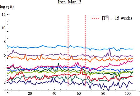
In particular in this work we wanted to see how the 2008 financial crisis affected a network structure. Typically, we consider the daily difference in logarithmic scale of the stock’s value, called return r_i . But we can consider the time resolution that best answers our questions.

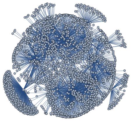
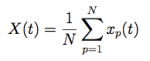
We considered a portfolio of N stocks, quoted simultaneously on the market in a time window T. Using the daily fluctuation of prices we evaluated the correlation coefficients between all stocks. These correlations form a matrix of values, that can be translated into a fully connected weighted graph. A fully connected graph is a graph where every node is connected to the others. Here, all the information resides in the weights. In this case the role of algorithms on graph is to extract meaningful weights, that are indeed correlations. We will in fact select a subset of relevant links.

We evaluated the correlation coefficients between the 500 Standard & Poor’s stock market indices, obtaining a symmetric matrix of numbers, -1  ≤ ρ_ij  ≤ 1, with 1 on the diagonal.

We confronted two time windows, respectively called 07 and 09: 1/1/1985 – 6/1/2007 and 1/1/1985 – 12/14/2009, separately for values at opening and closing time. The resulting sets are 4 fully connected weighted graphs, Opening 07 and 09 and Closing 07 and 09. The simple transformation that we performed on this matrix of correlations give us a weighted graph, we just need to define a distance, in order to have non negative numbers 0 ≤ d_ij ≤ 2. Now we have a fully connected graph, where every node has degree N -1.

How can we highlight the strongest correlations in this graph? The well known subgraph that we will extract is the minimum spanning tree. This object is a weighted undirected graph, which connects all the vertices together with the minimal total weighting for its edges. And, of course, it doesn’t have loops. The recursive algorithm that I performed on these matrices is called Prim’s algorithm. There are other algorithms that can find the minimum spanning tree of a graph, even if this graph is disconnected. But our case regards a fully connected graph, so Prim’s algorithm works fine. The result will be the same, no matter what vertex is our first vertex in analysis.

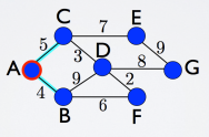
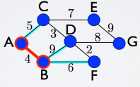
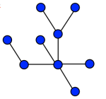
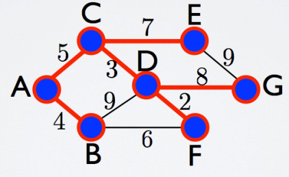
Let’s take a look at this example, a connected graph with some weights. Starting from the vertex A, in red in the picture before, we consider all its links (cyan), we evaluate and we select the one with the smaller number, that is 4. We can move now to the vertex B. We will have to add this vertex to our red selection, and evaluate all the other links, which connect my red part with the remaining vertices. Then again we will choose the smaller weight, that is 5, and select that link and the connected vertex C, and evaluate again which one to choose. The procedure goes on and on until we evaluated all the links and all the vertices are now red and connected to each other. Like in this picture below, where the red selection is the minimum spanning tree of the entire graph.

Another criterion that we used is basically a threshold criterion, we select all the links that correspond to a certain value, and above, of correlation. In this example if we want to select weights of value 5 and below (considering this weight as a distance), we will obtain 3 disconnected parts. Vertices A, B, C, D and F in one cluster and two separate vertices, E and G, which form two more clusters. As we can see, this rough criterion will probably give us disconnected parts, depending significantly on the chosen threshold. On the contrary the minimum spanning tree, by definition, is the spanning tree that connects all the vertices, and we never have disconnected part. Therefore there is something very interesting in this second criterion, which is the possibility of seeing the emergence of clusters, that are vertices highly correlated between each other.

What happened when we performed these filtering procedures on the correlation matrices of our stocks? We will see in the next post our interesting results! Stay tuned.

K-cores Decomposition of a Real Network

Let’s now consider a real network. The Internet is a very complex system and its rapid growth makes its graph representation very interesting, from a topological point of view. Many projects tried to map the Internet and this implies all kinds of difficulties. DIMES project has the peculiarity of being a collective effort, it is a distributed scientific research project, aimed to study the structure and topology of the Internet, with the help of a volunteer community. What you have to do to participate and become an Active Agent is to download a small program that will run in the background of your computer, consuming very little resources. The network considered for this post is the result of the data gathered from 2004 to 2007, it has 34563 vertices and 62960 edges, with a maximum degree of 2897. In particular this is the Autonomous System (AS) level of the Internet network. Each vertex represents an autonomous system and each edge is a connection between two AS. That is why it may seem small, but every vertex is a collection of routers and networks under the same domain or administrative entity.

Dimes AS Network Degree Distribution

I already mentioned here the first characteristic of complex networks, the scale invariance with the typical power-law distribution of degrees. We can see in the picture above that in this case we have indeed a power-law with an exponent of 2.5 and a long exponential tail.

We observed here that for a random graph we have a Poisson distribution of degrees and consequently an homogeneous topology. We may expect now something quite different. How does this k-cores decomposition look like? We can see below in red the distribution of vertices, and in blue the edges, that is the number of vertices and edges in each shell. It seems the opposite of what we saw for random graphs. Most vertices are in the lower shells, and few are very connected. The number of elements in each shell decreases with k. In particular the number of vertices decreases with k following a power-law with an exponent of 2.7.

Dimes Network with 34563 vertices and 62920 edges, k-cores decomposition

In the figure below these characteristics become even more clear. This very nice image is obtained with the LaNet-vi visualization tool, mentioned in the previous post and described here. The size of a vertex represents its degree and the color represents its coreness value (or the shell where the vertex is). This graph has clearly an heterogeneous topology, there is an evident hierarchy, most vertices are in the lower shells, pink and purple, whereas a limited number of vertices has an important role in the network, in the center of the picture. These red vertices are called hubs and they have a very large number of connections. Emergence of hubs is a consequence of the scale-free property of networks. Hubs can be found in many real networks and have a significant impact on the topology, but they cannot be observed in a random network, as we already saw.

How this network would resist to damages and attacks? We already saw that removing a random vertex in a network with an homogeneous topology like a random graph we probably would not cause much trouble, because those vertices have a similar role in the network, they are interchangeable. Here instead, we have a group of nodes that are essential, without one of them we would probably find our network divided in disconnected components or clusters. Here of course, removing a random element means to touch more likely one of the less important vertices, but we have a part of the network very sensitive and an attack towards one of the red vertices would have serious consequences. This example of an highly hierarchical network shows us why local failures don’t usually lead to catastrophic global failures. Scale-free networks are resilient with respect to random attacks, whereas targeted attacks are very effective.

k-cores decomposition visualization by LaNet-Vi

K-cores Decomposition of a Random Graph

We described what cores are and it is now time to see how a network looks like, once we performed the k-cores decomposition. There is a very interesting visualization tool for graphs called LaNet-vi and it is based on the k-cores decomposition, described in previous posts here and here. This visualization tool provides very nice images of large scale networks on a two-dimensional layout.

Let’s consider first a random graph with N vertices and M edges. A random graph is obtained by a stochastic process that starts with N vertices and no edges, and at each step adds one new edge chosen uniformly with probability p from the set of missing edges. The number of possible edges is N (N – 1), that is the number of edges of a complete graph. A random graph with N vertices and M edges has an average degree c = 2 M / N, and the degree distribution follows a Poisson probability distribution. As we saw before, the k-core decomposition depends strongly on how the edges are distributed among the vertices.

The theory of random graphs says that there is a critical threshold c(k): if c ≥ c(k) then the k-core exists and it is formed by a finite group of vertices. I generated several random graphs for c = 4, 7, 10 and I performed the k-cores decompositions, writing some code in C programming language. In the plot below we can see the number of edges (in blue) and the number of vertices (in red) that belong to a k-shell (the vertices and edges that belongs to the k-core but not to the (k+1)-core ) with a value of coreness k. The green small squares represent the theoretical values for random graphs, given c and N. If you are interested the code is available in my repository here under the KCores folder.

Random Graph with 10^5 vertices

How does this k-cores decomposition look like? And how is this useful? We notice that most of the vertices and edges belong to cores with high value of k. And also that the number of elements in a shell grows with k. And when c grows, new cores with larger k appear, as we expected from random graph theory. In the figure below these characteristics become even more clear. This very nice image is obtained with the LaNet-vi tool, mentioned above. This random graph has 1000 vertices and an average degree c = 10. The size of a vertex represents its degree and the color represents its coreness value (or the shell where the vertex is). This graph has clearly an homogeneous topology, there is no evidence of hierarchy, most of the vertices share the same role in the network (in red in the picture below). Often we read about the strenght of a network, that is how a network resists to damages or attacks. In this case, with an homogeneous structure, if we remove a random vertex or edge, we probably would not cause much trouble to this network, because most vertices are connected to each other and share the same role. This means that a random graph has a strong structure. And, obviously, this is the exact opposite of what we have in real networks.  But we will see what happens in real life in the next post!

k-cores decomposition visualization by LaNet-Vi

K-pruning Algorithm

We want to highlight in a graph some subsets with important connectivity properties, the cores. We described what these cores are in detail in a previous post. But how do we break down a graph in its cores? To partition the graph there is an interesting recursive algorithm, called k-pruning and I will describe here how it works. I also wrote some code in C programming language, to perform this decomposition on a general undirected graph, given its representation as a list of edges in a text file. 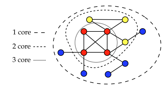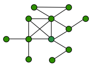If you are interested you can find this C code here in my repository (under kCores folder).Let’s now consider a cyclic undirected graph, green vertices in the figure above. From the definition of k-core we have that every vertex with degree ≥ k belongs to the k-core. We notice that every vertex in this graph has degree ≥ 1, thus the whole graph should be a 1-core.

The algorithm of the k-pruning says: remove recursively all vertices with degree < k, the remaining vertices belong to the k-core.  In order to have all the possible cores of the graph, we have to perform this recursive pruning for k going from the minimum degree of the graph to the maximum degree. In this case we have minimum 1 and maximum 6. According to this procedure, we can see that there are no isolated vertices, with degree < 1, thus the whole graph is a 1-core, as we already noticed.

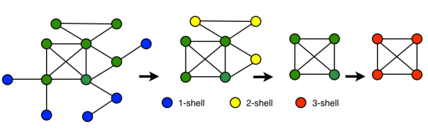
We now remove recursively all vertices with degree < 2, the vertices in blue in the figure above. We obtain the 2-core (remaining green vertices). The blue vertices belong to the 1-core but not to the 2-core, thus they are the 1-shell (see here for definitions and more details). Same happens for the vertices with degree < 3, in yellow in the figure above. They are removed recursively and we obtain the 2-shell, and the remaining vertices belong to the 3-core. We notice now that removing all vertices with degree < 4 we have nothing left. That means that the we have no more inner cores to find.

We did not perform the pruning for all values of allowed k, from minimum degree 2 to maximum degree 6. With degree 4 we already found no vertices left. This gives us an idea of how many and strong connections should be in a graph, in order to resist to a pruning with an high value of k. Therefore the core decomposition of a graph gives us very different results depending on the degree distribution.

K-cores Decomposition of a Graph

The Graph is a really beautiful and useful mathematical object, with many properties. Before introducing the k-cores, let’s describe shortly some basic principles. In general a graph is defined by a set of vertices and edges that connect pairs of vertices. Usually N represents the total number of vertices and M the number of edges. The degree is the fundamental characteristic. Every vertex has a degree, that is the number of edges that connect that vertex  with the others. With the same N and M we can build very different graphs, depending on the degree distribution, that represents how the edges are distributed among vertices.

Moreover graphs can be trees, which means without loops, or closed paths. Otherwise they are cyclic graphs, if they have at least one loop. The path from a vertex v to another vertex w is a sequence of connected vertices, where no edges or vertices are repeated. A loop is simply a path that starts and ends with the same vertex.

Example of a tree

A complete graph or fully connected graph, is a graph where every vertex is connected with all the others. If we have N total vertices, we will have all vertex with degree N – 1. Which means that we can go from everywhere to everywhere in just one step. Real networks usually do not have this super property, but they may have some highly connected parts. A clique in a graph is indeed a subset of vertices where every vertex has the maximum possible degree, in other words a complete graph inside another graph. In the example below in the 2-clique all vertices have degree 2, in the 3-clique all vertices have degree 3 and so on.

Example of n-clique

Let’s go further. A graph is k-connected if every pair of vertices is connected through at least k distinct paths, that do not share edges. This property is related to the strength of a network, in fact a k-connected network remains connected whenever fewer than k links are removed or broken.

Now we can finally introduce the k-core, also related to the strength of a network. The k-core is a subset of a graph where every vertex has degree ≥ k. Cores are nested, a graph can have a 2-core that includes a 3-core that includes a 4-core and so on. Every vertex of a graph has its coreness value, that represents the maximum k-core that contains it. In other words a vertex has coreness 3 if it belongs to the 3-core but not to the 4-core.  The k-shell is the subset of vertices with the same value of coreness. We can see now that cliques are always also cores. The opposite is not true, cores are not necessarily cliques.

In the example below we have a graph with its cores decomposition.  The maximum core has k = 3 even though the maximum degree of the graph is 6 (red vertex, top right corner of the square). Then we have the 2-core in yellow and red. The minimum core is the whole graph and it has k = 1, because there are some leaves, that are vertices with degree 1 (most blue vertices). It is now clear how cores are nested.

In the next post we will discuss and analyze the k-pruning algorithm, a recursive algorithm that allows us to break down systematically a graph in its cores.

Visits Time Series of a WikiNet

I built a WikiNet (a Wikipedia subset) starting from the article of a recently released movie, and I considered visits history of all articles in the WikiNet, one year before and after the movie release. We will see how the exogenous event, related to the movie release, influence the number of visits of the articles in the network.

I chose a well known movie, Iron Man 3 (released on May 3rd 2013 in USA), in order to have a lot of visitors and a lot of links in the network. I extracted the local neighborhood in Wikipedia as I described in a previous post and I obtained a non oriented graph. Of this graph I considered the central page, all its 461 first neighbors (FN) and just a random selection of 1 000 effectively second neighbors (SN), because some SN could be already FN. I had to restrict my analysis to a subset of articles for computational limitations. Downloading and processing time series for 24 months and for around 4 000 articles was far beyond my possibilities of time and computing power. Nevertheless my analysis is performed on a significant data set.

I considered a the time window of 24 months, and for each article I considered the weekly average and its logarithmic value. First of all I had to remove the effect of the weekly pattern of Wikipedia articles, described in this post, a global and regular fluctuation. Second, I had to reduce the differences among articles, because their typical average number of visits can be very different, and considering the logarithmic value is a valid choice in cases like this.

First Neighbors

Second Neighbors

How to Build a WikiNet

There are almost 5 million articles in English Wikipedia only, as I wrote in a previous post (Wikipedia as a Complex Network). As you may imagine, analyzing the whole dataset of the Wikipedia network needs some computational power. I wrote several functions and code lines in Mathematica to analyze a small part of this network. For those who want more details, in this repository here there are the Mathematica notebooks. These functions photograph the local neighborhood of a chosen Wikipedia article. First, we select an article that will be the central page of a Wikipedia subgraph, that I called WikiNet, to make it a bit shorter. Second, we decide the depth of this subgraph, but usually with depth 2 we are already considering a large dataset. These functions then browse and store the current subgraph within two-clicks distance starting from the central page. In this procedure I selected only links towards other English Wikipedia articles, excluding special pages, portals, disambiguation pages et similia.

Initially I had a directed graph, not necessarily a tree because some first neighbors might be linked to some other first neighbors or the central page. But I considered outdegrees and indegrees just as degrees, without orientation. Therefore the WikiNet is a simple graph, that is a not-oriented graph without selfoloops and multiedges. I considered then the central page, all its first neighbors (FN, articles one-click away from the central page) and all second neighbors (SN, articles one-click away from all FN).

Let’s consider for instance the WikiNet centered in the “Cloud_Atlas_(film)” article in Wikipedia. This graph is formed by N = 2023 nodes (pages) and M = 2287 edges (links).  With the following instructions in Mathematica it is possible to visualize the undirected graph, where CloudGraph is a list of all edges.

Structure and topology of this graph are clearly influenced by the way these functions extract the network, this give us a rough (but still effective) outline of the local image of the entire Wikipedia network. Which approximations are we considering? For all first neighbors and the central page I extracted the correct outdegree but partial information on indegrees. For all second neighbors I have partial indegrees and no idea of the outdegrees, for instance all those nodes that are packed in groups with only one link, they are clearly my network border. As I said before I had to limit the exploration to reduce computational costs, not really for the graph itself but for the visits history analysis that will follow (in future posts).

To have a quantitative idea let’s look at the degree distribution. This plot describes how connections are distributed in this WikiNet. There is a large number of articles with really few links (blue dots on the left) and a small number of articles with many links (on the right). The average degree in this network is 2.2, this confirms that we have a significative number of articles on the border of our subset of Wikipedia.

Wikipedia Visits Global Behavior

I tried to understand and characterize Wikipedia visits time series (also in this post Wikipedia Visits Time Series). I analyzed a random sample of English Wikipedia articles, I considered a first set of 1 000 pages and a second set of 10 000 pages. I downloaded and cleaned all their visits history for 12 months (first pages set), and for 2 months (second pages set). Looking at the data I observed two really interesting global behaviors, with two different time scales. Let’s look at the first data set, in the following plot we have the average daily visits X ( t ) for a year, that is the mean over all the N pages in the set for a certain day.

The first global behavior has a scale of a few months, that is a global decrease of visits during summer months and Christmas days. This low frequency fluctuation can be interpreted as a seasonal effect. It seems reasonable that people visit Wikipedia with less continuity during summer months. There is also a significant average decrease of visits around Christmas (red tick mark in the plot). Also reasonable, since the majority of readers is located in the Northern Hemisphere and Western World (according to Wikimedia Statistics we have main visitors origin: US 36%, UK 10.8%, Canada 6%, India 5%, Australia 3.3%, Germany 2.0%, Philippines 1.7%, Brazil 1.1%, Netherlands 1.1%, France 1.0%, Sweden 1.0%, Italy 0.9% … ). Which can explain the 15% decrease of visits during Christmas holidays  and summer months.

Daily visits of English Wikipedia pages from 08/2012 to 07/2013. Average value over a set of 1000 random articles.

What about these high frequency fluctuations? The second global behavior has a scale of  a few days. Let’s look at these fluctuations in a smaller time window. In the second plot we can see the average daily visit (but normalized this time) over a set of 10 000 random articles, for only 60 days. The blue and the dark red lines are the data (two sub-sets). The light red line is a sinus function, with a period of 7 days.

Average daily visits for 10000 random English Wikipedia articles, for two months.

I interpreted this result as a weekly pattern, in fact periodic minima correspond to weekend days. Which means that Wikipedia is usually consulted more during working days! Did you expect that?

Wikipedia Visits Time Series

Wikipedia is currently maintained by a non-profit organization called Wikimedia Foundation which has the goal of encouraging the growth, development and distribution of free, multilingual content. Because of its intent, not only does Wikimedia make the content of its Wikis available through specific Websites but also through dumps of their whole data that can be downloaded by end users (here). Each request of a page, whether for editing or reading, is collected and stored for several languages editions of Wikipedia. These data are available in files of 90 ÷ 120 MB for every hour of the day. Which means that a whole day could be 3 GB. A simpler way to access these data, since we often have computational limitations, is the Mitzuas’s project, which provides for a given Wikipedia article all its visits history per day since December 2007. For every page there is a JSON format file for each requested month. There is also a nice tool that allows you to visualize a page visits history (90 consecutive days at most).

Main Page visits on January 2015

To download and process automatically these data I wrote several functions and code lines in Mathematica programming language, and I obtained in the end clean and correct time series. For those who want more details, in this repository here there are the Mathematica notebooks. From now on, in this blog, I will always mean with Wikipedia pages only English Wikipedia articles, excluding special pages such as Main Page, Portal pages, Category pages, Project pages and others.

After downloading and cleaning the data, I tried to understand and characterize the visits time series of Wikipedia pages. I decided to restrict my analysis to articles related to movies, everybody loves cinema and I am not an exception. Wikipedia pages are already extremely heterogenous in nature and as a consequence in behavior. Usually visits of a page fluctuate a lot around its typical average and different pages can have very different averages. This typical value can represent a measure of the popularity of that page. Focusing on a specific category could help us in reducing effects that are difficult to understand.

We can see below an example of relatively stationary articles, two well known movies. The number of daily visits fluctuates around a typical value, nothing particularly strange happens in a year. There is no particular reason for people to visit these pages during this time. Just the usual. The access to these articles is not strictly stationary (as we studied in class), but considering the rather random behavior of web users, this is how much constant it can get.

Different story for different movies. We can see below the daily visits history for two popular movies, two beloved Christmas stories.  I truncated the red peak to keep details in the baseline. Something definitely happened. When talking about movies, understand a possible origin of a bursty activity may be easier, then considering articles of other categories. These films were probably aired on TV. This example describes how an exogenous event looks like. Something outside the net happened, and we can see how it clearly affects the number of visitors. The movie “A Christmas Story” had a peak of 245 034 visits on December 25th 2012, when its baseline usually fluctuates around 1 000 daily visits. Same thing, with a smaller peak of 12 550 daily visits, happened to the page “The Nightmare Before Christmas”, that usually fluctuates around 2 000 daily visits.

Christmas movies on Christmas days

In conclusion with this first approach to the data I saw that generally daily visits of a page fluctuate, often considerably, around a typical average, that depends strongly on the popularity of that page. Moreover this typical average may vary around very different values for each page. The system is very heterogenous, with strong natural fluctuations. And sometimes an exogenous event occurs, the number of visits explodes and after a while everything goes back to normal.

Wikipedia as a Complex Network

Since its inception Wikipedia has been gaining popularity and nowadays it is consistently ranked in the top 10 most popular sites according to Alexa (currently at 7th place). As of January 2015, it is comprised of more than 5 million of articles on a wide variety of subjects written in more than 200 languages. The number of articles on Wikipedia has been growing exponentially since its creation in 2001. This growth is mainly driven by the exponential increase in the number of users contributing new articles, indicating the importance of the Wikipedias open editorial policy in the current success (more technical details can be found here).

English Wikipedia has 9.5 billion page views per month, the number of articles is about 4.8 million and it grows of 7% every year (see here and here, very nice Wikimedia statistics). It is a complex network, with scale-free properties and power law distribution of degrees (more technical details here). Degree distributions, growth, topology, clustering and path length are common characteristics among different language versions of Wikipedia.

“Social Network Analysis Visualization” by Calvinius

Scale-free systems are one of the reasons why I decided to study Physics at University. I was reading “Chaos” by James Gleik, and it was kind of mind-blowing. I was eighteen and I had to decide what to do with my unclear skills in many things that I liked, as everyone. But those things… were exciting in a completely new way. “Scale-free” means that if you look at a system at a small and large scale, you would not be able to say which is which (see also scale invariance). Let’s go back to Wikipedia, the essential property of scale-free networks is having many nodes with few connections and few nodes with many connections, that is the power-law distribution  of degrees.

Usually complex networks such as social networks have also a small diameter of the corresponding graph of social connections. The diameter of a graph is the longest shortest path (or longest distance) that connects every pair of node. This property is related to the well known phenomenon of six-degree separation, that was proved with the social experiment conducted by Stanley Milgram before Internet was born (here). In other words, in a social network everyone can be reached by everyone within six steps of social connections. But every network has his particular degree of separation.

What happens in a network like Wikipedia?

In an interesting work (here) I found that they measured the average path length (or average distance between two nodes) of English Wikipedia and they found a value of almost 3 links, when considering the undirected graph (which means that every link is considered accessible in both directions even though it is not). The average path length si instead almost 5 when considering the directed graph (where every link has a direction).

I found on the Internet a nice tool in a beta version (degreesofwikipedia.com), where you can know the degree of separation (or distance) between two Wikipedia pages of your choice. Have fun!